Welcome!
Introduction
Variations of the Traveling Salesman Problem (TSP) have existed since the 1800s. Generally speaking, the problem can be stated as:Given a list of cities and the distances between each pair of cities, what is the shortest possible route that visits each city exactly once and returns to the origin city?
In essence, this question is asking us (the salesman) to visit each of the cities via the shortest path that gets us back to our origin city. We can conceptualize the TSP as a graph where each city is a node, each node has an edge to every other node, and each edge weight is the distance between those two nodes.
The first computer coded solution of TSP by Dantzig, Fulkerson, and Johnson came in the mid 1950’s with a total of 49 cities. Since then, there have been many algorithmic iterations and 50 years later, the TSP problem has been successfully solved with a node size of 24,978 cities! Multiple variations on the problem have been developed as well, such as mTSP, a generalized version of the problem and Metric TSP, a subcase of the problem.
The original Traveling Salesman Problem is one of the fundamental problems in the study of combinatorial optimization—or in plain English: finding the best solution to a problem from a finite set of possible solutions. This field has become especially important in terms of computer science, as it incorporate key principles ranging from searching, to sorting, to graph theory.
Real World Applications
However, before we dive into the nitty gritty details of TSP, we would like to present some real-world examples of the problem to illustrate its importance and underlying concepts. Applications of the TSP include:
Click on an example to the left for more information!
- Santa delivering presents.
- Fulfilling an order in a warehouse.
- Designing and building printed circuit boards.
- Analyzing an X-Ray.
- GPS satellite systems.
- School bus scheduling.
Finding Solutions – Exact vs. Approximation
The difficulty in solving a combinatorial optimization problem such as the TSP lies not in discovering a single solution, but rather quickly verifying that a given solution is the optimal solution. To verify, without a shadow of a doubt, that a single solution is optimized requires both computing all the possible solutions and then comparing your solution to each of them. We will call this solution the Exact solution. The number of computations required to calculate this Exact solution grows at an enormous rate as the number of cities grow as well. For example, the total number of possible paths for 7 cities is just over 5,000, for 10 cities it is over 3.6 million, and for 13 cities it is over 6 billion. Clearly, this growth rate quickly eclipses the capabilities of modern personal computers and determining an exact solution may be near impossible for a dataset with even 20 cities. We will explore the exact solution approach in greater detail during the Naïve section.
The physical limitations of finding an exact solution lead us towards a very important concept – approximation algorithms. In an approximation algorithm, we cannot guarantee that the solution is the optimal one, but we can guarantee that it falls within a certain proportion of the optimal solution. The real strength of approximation algorithms is their ability to compute this bounded solution in an amount of time that is several orders of magnitude quicker than the exact solution approach. Later on in this article we will explore two different approximation algorithms,
Nearest Neighbor and Christofide’s Algorithm, and the many facets of each approach.
The Naïve Approach
Speed:
Nearest Neighbor
Speed:
Christofides Algorithm
Algorithm Analysis
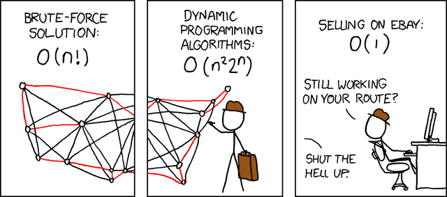
Throughout the article we have introduced several different algorithms for solving the Traveling Salesman Problem. The use cases for these algorithms is primarily based on their runtime performance vs error % tradeoff. So, during this section we will compare how the algorithms compare to one another. Less Cities More CitiesWhile the Naïve and dynamic programming approaches always calculate the exact solution, it comes at the cost of enormous runtime; datasets beyond 15 vertices are too large for personal computers. The most common approximation algorithm, Nearest Neighbor, can produce a very good result (within 25% of the exact solution) for most cases, however it has no guarantee on its error bound. That said, Christofides algorithm has the current best error bound of within 50% of the exact solution for approximation algorithms. Christofides produces this result in a “good” runtime compared to Naïve and dynamic, but it still significantly slower than the Nearest Neighbor approach.
In the chart above the runtimes of the naive, dynamic programming, nearest neighbors, and Christofides’ are plotted. The x-axis represents the number of cities that the algorithm works on while the y-axis represents the worst-case amount of calculations it will need to make to get a solution. As you can see, as the number of cities increases every algorithm has to do more calculations however naive will end up doing significantly more. Note how with 20 cities, the naive algorithm is 5,800,490,399 times slower than even the minimally faster dynamic programming algorithm.
Closing Thoughts
We would like to thank Dr. Heer, Matthew Conlen, Younghoon Kim, and Kaitlyn Zhou for their contributions to CSE 442, the UW Interactive Data Lab, Idyll, and much more. This article would not have been possible without their support and guidance.
Authors
Roy MatthewKevin Zhao
Divya Cherukupalli
Kevin Pusich
Sources, References, and Links:
Inspiration from Idyll articles: Flight, Barnes Hut
Eulerian tourChristofides solver
General TSP code
graph-lib
TSP History
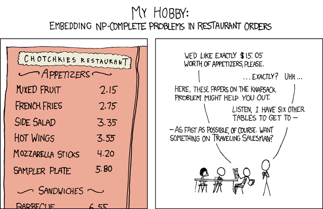
Thanks to xkcd for these comical comics as well!