Stepping Into the Filter
Understanding the Edge Detection Algorithms in Your Smartphone

What Is Edge Detection?
Have you ever wondered how Facebook can recommend who to tag in a photo you just posted? Or how smartphones sharpen the image around your face when you take a selfie? The answer is a little magic, a tad mundane, and a bit of math.
Edge Detection is a process which takes an image as input and spits out the edges of objects in the photo. The algorithm has crossed domains, and is used in areas from computer vision to robotics. The family of Edge Detection algorithms is large and still growing. We will take you through some of the core algorithms used today. Sit back, relax, and Step Into the Filter.
Representation of a Picture
intensity: 0
People say, “A picture is worth a thousand words.” And pictures are made of thousands of pixels. So let’s devote some words to talking about pixels!
Pixels are tiny boxes full of color which you cannot see with the naked eye. A pixel’s color is defined by it’s RGB (Red, Green, Blue) tuple. Each color you see is a combination of red, green, and blue. And each element in the tuple ranges from 0 to 255: 0 is no color, 255 is full saturation. Each unique tuple can also be identified by its hexadecimal (Hex) value. Try out the color selector to see what the RGB tuple is for a variety of colors. If you are curious, the fourth channel, A, stands for “Alpha” which is a measure of transparency. Our edge detection algorithms do not use this fourth channel.
Notice how the intensity value below the color picker changes as you select different colors. We will talk more about intensity and how it is calculated in the next section.
Color Intensity


The first step in Edge Detection algorithms is to determine the intensity of an RGB tuple. Intensity is a measure of a pixel’s saturation. Which is more intense, a pixel which is full red (255, 0, 0) or a pixel which is full green (0, 255, 0)? Trick question (we hate those too)! They are the same intensity!
We need a way to map from RGB tuples to a single measure of intensity. So to simplify the problem, we will convert our images to black and white (grayscale). The scale from black to white is a measure of intensity. The standard equation for converting to grayscale uses some magic (but standard) numbers which allows you to differentiate between colors.
Graphing Intensity
Let’s start with a rectangular picture that contains a smooth gradient from black to white. Pretend that the image is 1 pixel high and 1000 pixels long- in our example we have enlarged the picture so you can see it.
Next, we draw a graph of the intensity of each pixel -- black has the lowest intensity and white has the highest intensity. Run your cursor over the graph to the right. Notice how in the middle of the gradient, the intensity suddenly changes. This change represents an edge! We’ll make a proper Edge Detector out of you in no time.
Sobel Edge Detection
But how can we easily find where the intensity changes? One solution is to graph the slope of our intensity curve. For those readers who know calculus, this is the first derivative.
When we graph the slope of the intensity curve, we see a peak. This peak tells us where the edge is! In particular, this method of edge detection is how the Sobel algorithm works.
Kernels
Vertical Sobel Kernel
A list of pixel intensity is not a continuous function, so we’ll have to approximate the derivative. But how do we approximate a derivative over a 2D plane? We use a convolution.
Before we dive into convolutions we need to explain a helpful tool, the kernel. We can think of a kernel as a small matrix. The center-most box of the matrix is the anchor. Look at the matrix on the right, this is the kernel used for the vertical portion of the sobel algorithm. The anchor is 0. We’ll use this kernel to do some calculations on an image.
Convolutions
Pixel Data
Dealing with the edges and corners of images can be difficult, because of missing pixels around the anchor. Above, we ignore edges and corners for simplicity and continue with our convolution. Advanced techniques for handling these edge cases include mirroring the image across the edge, using pixels from the other side of the image, and duplicating the edge pixels. The edge detection algorithms at the end of this article (for you to play with) mirror the pixels across all edges and corners.
Selection
*
Kernel
=
Result
Take a look at the example "picture" to the right. Hover your mouse over the pixel data to see the convolution calculations. In the above matrixes, the left is a view of your convolution selection, the middle is our kernel, and the right is the resultant matrix. Our algorithms at the end of the article start the convolution in the upper left corner and move left to right, top to bottom, through each pixel in the image.
Sobel Returns
Horizontal Sobel Kernel
Vertical Sobel Kernel
Now that we have those derivatives, we can use them to find edges. Using the Sobel method, we can define the strength of the edge as a combination of the horizontal and vertical derivatives. We can also find the orientation of that edge using the arctangent. With this information, you can then find the strength and orientation of edges in a picture.
To draw the edges detected by the Sobel algorithm, your canvas should reflect how strong the edges are with a darker color and which direction the edges are going via the orientation.
Laplacian Method
So far our edge detection method is simple. Every time we see a peak in the slope of the intensity, we mark that as an edge. But what about small peaks, are those edges or just small color changes due to shadows? How can we determine whether a peak represents an edge or noise?
One solution is to graph the slope of our first derivative curve. The key idea is that when the first derivative curve is rising, the slope is positive. When the curve is descending, the slope is negative.
In our first derivative curve, the slope slowly increases at the start of the gradient. Halfway through the rise to our peak, the slope sharply increases. Then, as it approaches the peak, the slope decreases again.
At the very peak of our first derivative, the slope is 0. We have stopped ascending the mountain and are resting before descent.
On the way down the peak, we start with a slow descent, the slope decreasing more quickly around the middle. Then, as we approach the last pixel, the slope slows.
Now we have a graph of what is called the second derivative. The point where the graph crosses 0 marks our edge. This method of detecting edges is how the Laplacian algorithm works. Back to our initial question of what makes a peak an edge or noise, we set an arbitrary threshold value to separate edges from the background noise. If the magnitude of the second derivative (for both sides surrounding 0) is large enough, we have an edge.
Laplacian kernel
In practice, the Laplacian method uses a kernel which can approximate the second derivative. The Laplacian method only requires one kernel because rotating the Laplacian kernel gives you the same kernel back. Thanks symmetry!
Pixel Data
Try out the three kernels we’ve defined so far: Horizontal Sobel, Vertical Sobel, and Laplacian.
Selection
*
Kernel
=
Result
Sobel vs Laplacian

We have two methods for detecting edges: Sobel and Laplacian. Sobel uses horizontal and vertical kernels, while Laplacian uses one symmetrical kernel.
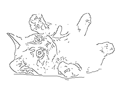
If images could talk, I bet they would have great stories -- full of colorful language and loud noises. Noise is a feature of all images. Noise could be a cat’s fur -- all those soft pieces of hair define edges against each other. Noise could also be a function of an image’s compression, picking up artifacts and other products of encoding. Both the Laplacian and Sobel methods are impacted by noise in the image.
Gaussian Smoothing
 Laplacian of Gaussian
One way to deal with noise is to smooth out the image. We can do a convolution using a kernel of Gaussian values to blur or smooth the image. By blurring the image, we reduce the level of detail -- so it looks fuzzy. Our Laplacian and Sobel methods will pick up fewer edges, but also less noise.
Canny Edge Detector
 Canny Edge Detection
The Canny edge detector combines many different optimizations. It involves four steps:
- Smooth the image using a Gaussian filter to reduce noise.
- Figure out where the intensity changes the quickest.
- Filter out the local maximum and minimum values with a high and low pass filter thresholds.
- Determine strong edges from weak ones, using values of intensity, and link the strong edges together.
(If you are curious, you can read more here).